Response Surface Designs
In this section, the following kinds of response surface designs will be described:
Hint
All available designs can be accessed after a simple import statement:
>>> from pydoe import (
...     bbdesign,
...     ccdesign,
...     doehlert_shell_design,
...     doehlert_simplex_design,
... )
Box-Behnken (bbdesign)

Box-Behnken designs can be created using the following simple syntax:
bbdesign(n, center)
where n is the number of factors (at least 3 required) and center is the number of center points to include. If no inputs given to center, then a pre-determined number of points are automatically included.
Examples
The default 3-factor Box-Behnken design:
>>> bbdesign(3)
array([[-1., -1.,  0.],
       [ 1., -1.,  0.],
       [-1.,  1.,  0.],
       [ 1.,  1.,  0.],
       [-1.,  0., -1.],
       [ 1.,  0., -1.],
       [-1.,  0.,  1.],
       [ 1.,  0.,  1.],
       [ 0., -1., -1.],
       [ 0.,  1., -1.],
       [ 0., -1.,  1.],
       [ 0.,  1.,  1.],
       [ 0.,  0.,  0.],
       [ 0.,  0.,  0.],
       [ 0.,  0.,  0.]])
A customized design with four factors, but only a single center point:
>>> bbdesign(4, center=1)
array([[-1., -1.,  0.,  0.],
       [ 1., -1.,  0.,  0.],
       [-1.,  1.,  0.,  0.],
       [ 1.,  1.,  0.,  0.],
       [-1.,  0., -1.,  0.],
       [ 1.,  0., -1.,  0.],
       [-1.,  0.,  1.,  0.],
       [ 1.,  0.,  1.,  0.],
       [-1.,  0.,  0., -1.],
       [ 1.,  0.,  0., -1.],
       [-1.,  0.,  0.,  1.],
       [ 1.,  0.,  0.,  1.],
       [ 0., -1., -1.,  0.],
       [ 0.,  1., -1.,  0.],
       [ 0., -1.,  1.,  0.],
       [ 0.,  1.,  1.,  0.],
       [ 0., -1.,  0., -1.],
       [ 0.,  1.,  0., -1.],
       [ 0., -1.,  0.,  1.],
       [ 0.,  1.,  0.,  1.],
       [ 0.,  0., -1., -1.],
       [ 0.,  0.,  1., -1.],
       [ 0.,  0., -1.,  1.],
       [ 0.,  0.,  1.,  1.],
       [ 0.,  0.,  0.,  0.]])
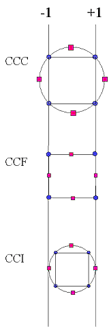
Central Composite (ccdesign)

Central composite designs can be created and customized using the syntax:
ccdesign(n, center, alpha, face)
where
nis the number of factors,centeris a 2-tuple of center points (one for the factorial block, one for the star block, default (4, 4))alphais either "orthogonal" (or "o", default) or "rotatable" (or "r")faceis either "circumscribed" (or "ccc", default), "inscribed" (or "cci"), or "faced" (or "ccf").

The two optional keyword arguments alpha and face help describe how the variance in the quadratic approximation is distributed. Please see the NIST web pages if you are uncertain which options are suitable for your situation.
Note
- 'ccc' and 'cci' can be rotatable designs, but 'ccf' cannot.
- If
faceis specified, whilealphais not, then the default value ofalphais 'orthogonal'.
Examples
Simplest input, assuming default kwargs:
>>> ccdesign(2)
array([[-1.        , -1.        ],
       [ 1.        , -1.        ],
       [-1.        ,  1.        ],
       [ 1.        ,  1.        ],
       [ 0.        ,  0.        ],
       [ 0.        ,  0.        ],
       [ 0.        ,  0.        ],
       [ 0.        ,  0.        ],
       [-1.41421356,  0.        ],
       [ 1.41421356,  0.        ],
       [ 0.        , -1.41421356],
       [ 0.        ,  1.41421356],
       [ 0.        ,  0.        ],
       [ 0.        ,  0.        ],
       [ 0.        ,  0.        ],
       [ 0.        ,  0.        ]])
More customized input, say, for a set of computer experiments where there isn't variability so we only need a single center point:
>>> ccdesign(3, center=(0, 1), alpha="r", face="cci")
array([[-0.59460356, -0.59460356, -0.59460356],
       [ 0.59460356, -0.59460356, -0.59460356],
       [-0.59460356,  0.59460356, -0.59460356],
       [ 0.59460356,  0.59460356, -0.59460356],
       [-0.59460356, -0.59460356,  0.59460356],
       [ 0.59460356, -0.59460356,  0.59460356],
       [-0.59460356,  0.59460356,  0.59460356],
       [ 0.59460356,  0.59460356,  0.59460356],
       [-1.        ,  0.        ,  0.        ],
       [ 1.        ,  0.        ,  0.        ],
       [ 0.        , -1.        ,  0.        ],
       [ 0.        ,  1.        ,  0.        ],
       [ 0.        ,  0.        , -1.        ],
       [ 0.        ,  0.        ,  1.        ],
       [ 0.        ,  0.        ,  0.        ]])
Doehlert Design (doehlert_shell_design, doehlert_simplex_design)
An alternative and very useful design for second-order models is the uniform shell design proposed by Doehlert in 1970 1.
Doehlert designs are especially advantageous when optimizing multiple variables, requiring fewer experiments than central composite designs, while providing efficient and uniform coverage of the experimental domain.
The Doehlert design defines a spherical experimental domain and emphasizes uniform space filling. Although it is not orthogonal or rotatable, it is generally sufficient for practical applications.
For two variables, the Doehlert design consists of a center point and six points forming a regular hexagon, situated on a circle. The total number of experiments is given by: $$ N = k^2 + k + C_0 $$ where
- \(k\) = number of factors (variables)
- \(C_0\) = number of center points
Two implementations are included:
doehlert_shell_design: uses a shell-based spherical approach with optional center points.doehlert_simplex_design: uses a simplex-based method to uniformly fill the design space.
Examples
Create a Doehlert design with 3 factors and 1 center point using the shell approach:
>>> doehlert_shell_design(3, num_center_points=1)
array([[ 0.       ,  0.       ,  0.        ],
       [ 1.       ,  0.       ,  0.        ],
       [-0.5      ,  0.8660254,  0.        ],
       [-0.5      , -0.8660254,  0.        ],
       [ 0.8660254,  0.5      ,  0.        ],
       [ 0.8660254, -0.5      ,  0.        ],
       ...                                  ])
Create a Doehlert design using the simplex approach for 3 factors:
>>> doehlert_simplex_design(3)
array([[ 0.      ,  0.       , 0.        ],
       [ 1.      ,  0.       , 0.        ],
       [ 0.      ,  0.8660254, 0.        ],
       [ 0.      ,  0.5      , 0.81649658],
       [-1.      ,  0.       , 0.        ],
       [ 0.      , -0.8660254, 0.        ],
       ...                                ])
Note
Doehlert designs are recommended for response surface modeling when good space coverage and fewer experimental runs are desired.
More Information
If the user needs more information about appropriate designs, please consult the following articles:
There is also a wealth of information on the NIST website about the various design matrices that can be created as well as detailed information about designing/setting-up/running experiments in general.