Randomized

In this section, the following kinds of randomized designs will be described:

• Latin-Hypercube
• Orthogonal Array-based Latin Hypercube
• Sliced Latin Hypercube
• Nested Latin Hypercube
• Maximin Distance Design
• Minimax Distance Design
• Maximum Projection (MaxPro) Design
• Nearly Orthogonal Latin Hypercube
• Random K-Means
• Random Uniform

>>> from pydoe import (
...     lhs,
...     oa_lhd,
...     random_k_means,
...     random_uniform,
...     sliced_lhs,
...     nested_lhs,
...     maximin_design,
...     minimax_design,
...     maxpro_design,
...     nearly_orthogonal_lhs,
... )

Latin-Hypercube (lhs)¶

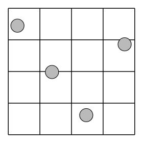
Latin-hypercube designs can be created using the following simple syntax:

lhs(n, [samples, criterion, iterations])

where

• n: an integer that designates the number of factors (required)
• samples: an integer that designates the number of sample points to generate for each factor (default: n)

• criterion: a string that tells lhs how to sample the points (default: None, which simply randomizes the points within the intervals):

• "center" or "c": center the points within the sampling intervals

• "maximin" or "m": maximize the minimum distance between points, but place the point in a randomized location within its interval
• "centermaximin" or "cm": same as "maximin", but centered within the intervals
• "correlation" or "corr": minimize the maximum correlation coefficient
• "lhsmu" : Latin hypercube with multifimensional Uniformity. Correlation between variable can be enforced by setting a valid correlation matrix. Description of the algorithm can be found in Latin hypercube sampling with multidimensional uniformity.

The output design scales all the variable ranges from zero to one which can then be transformed as the user wishes (like to a specific statistical distribution using the scipy.stats.distributions ppf (inverse cumulative distribution) function. An example of this is shown below.

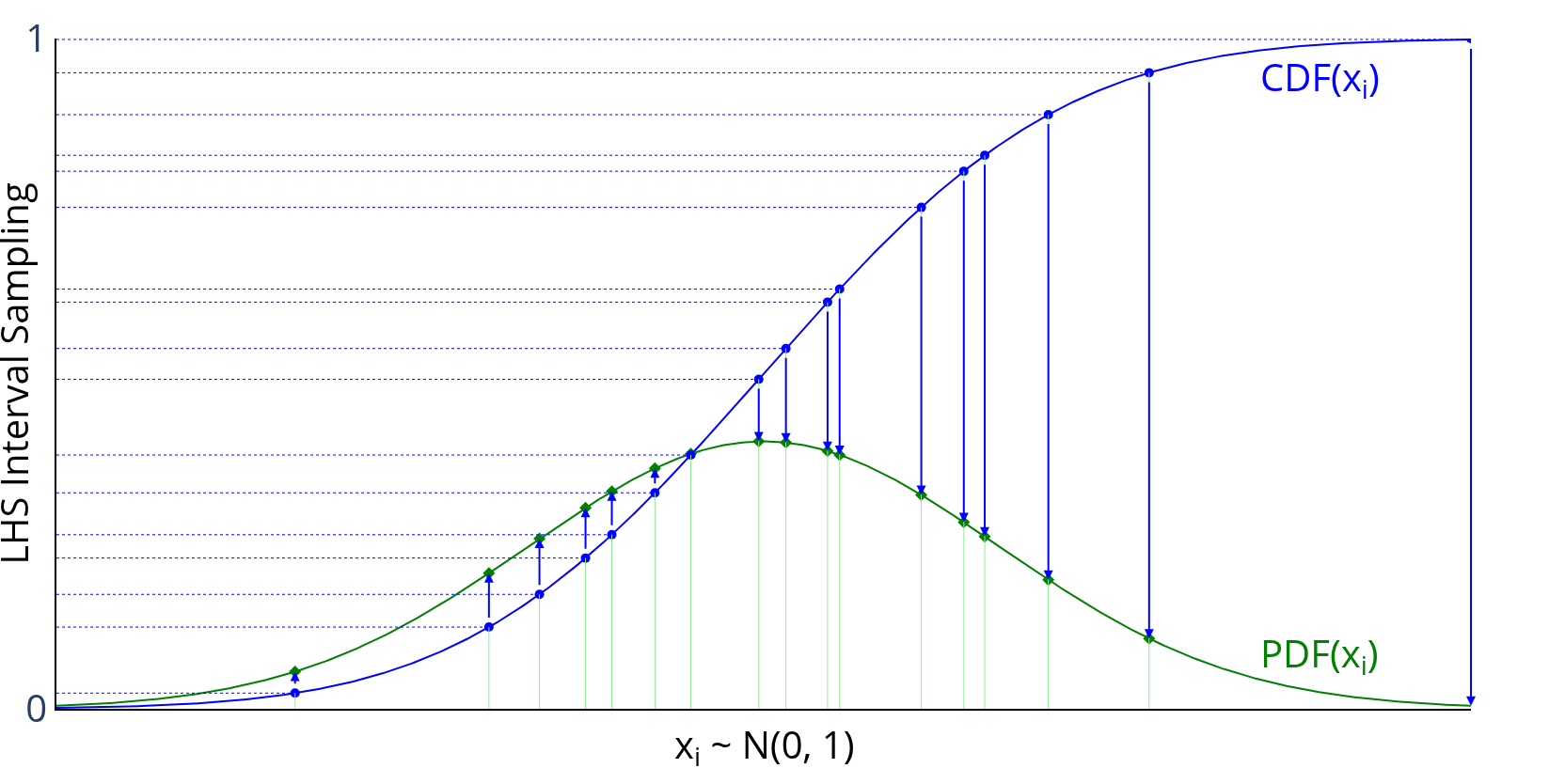
For example, if I wanted to transform the uniform distribution of 8 samples to a normal distribution (mean=0, standard deviation=1), I would do something like:

>>> from scipy.stats.distributions import norm
>>> lhd = lhs(2, samples=5)
>>> lhd = norm(loc=0, scale=1).ppf(lhd)  # (1)!

1. this applies to both factors here

Graphically, each transformation would look like the following, going from the blue sampled points (from using lhs) to the green sampled points that are normally distributed:

Examples¶

A basic 4-factor latin-hypercube design:

>>> lhs(4, criterion="center")
array([[ 0.875,  0.625,  0.875,  0.125],
       [ 0.375,  0.125,  0.375,  0.375],
       [ 0.625,  0.375,  0.125,  0.625],
       [ 0.125,  0.875,  0.625,  0.875]])

Let's say we want more samples, like 10:

>>> lhs(4, samples=10, criterion="center")
array([[ 0.05,  0.05,  0.15,  0.15],
       [ 0.55,  0.85,  0.95,  0.75],
       [ 0.25,  0.25,  0.45,  0.25],
       [ 0.45,  0.35,  0.75,  0.45],
       [ 0.75,  0.55,  0.25,  0.55],
       [ 0.95,  0.45,  0.35,  0.05],
       [ 0.35,  0.95,  0.05,  0.65],
       [ 0.15,  0.65,  0.55,  0.35],
       [ 0.85,  0.75,  0.85,  0.85],
       [ 0.65,  0.15,  0.65,  0.95]])

Customizing with Statistical Distributions¶

Now, let's say we want to transform these designs to be normally distributed with means = [1, 2, 3, 4] and standard deviations = [0.1, 0.5, 1, 0.25]:

>>> design = lhs(4, samples=10)
>>> from scipy.stats.distributions import norm
>>> means = [1, 2, 3, 4]
>>> stdvs = [0.1, 0.5, 1, 0.25]
>>> for i in xrange(4):
...     design[:, i] = norm(loc=means[i], scale=stdvs[i]).ppf(design[:, i])
...
>>> design
array([[ 0.84947986,  2.16716215,  2.81669487,  3.96369414],
       [ 1.15820413,  1.62692745,  2.28145071,  4.25062028],
       [ 0.99159933,  2.6444164 ,  2.14908071,  3.45706066],
       [ 1.02627463,  1.8568382 ,  3.8172492 ,  4.16756309],
       [ 1.07459909,  2.30561153,  4.09567327,  4.3881782 ],
       [ 0.896079  ,  2.0233295 ,  1.54235909,  3.81888286],
       [ 1.00415   ,  2.4246118 ,  3.3500082 ,  4.07788558],
       [ 0.91999246,  1.50179698,  2.70669743,  3.7826346 ],
       [ 0.97030478,  1.99322045,  3.178122  ,  4.04955409],
       [ 1.12124679,  1.22454846,  4.52414072,  3.8707982 ]])

Orthogonal Array-based Latin Hypercube (oa_lhd)¶

oa_lhd builds a Latin hypercube design from a symmetric orthogonal array using Tang's (1993) construction. Each column of the result is a permutation of all N cell midpoints, jittered within the cell, while respecting the level structure of the orthogonal array. This gives better two-dimensional uniformity than a plain random Latin hypercube.

>>> oa_lhd(oa, [seed])

where

• oa: a 2D array-like OA(N, k, s, 2) with integer levels 0, ..., s - 1, each level appearing exactly N / s times in every column (e.g. from get_orthogonal_array)
• seed: an integer or np.random.Generator for reproducibility (default: None)

The output design scales to the unit hypercube \([0, 1)^k\) with N cells.

Examples¶

>>> from pydoe import get_orthogonal_array, oa_lhd
>>> oa = get_orthogonal_array("L9(3^4)")
>>> oa_lhd(oa, seed=0)
array([[0.31813099, 0.17127347, 0.03330132, 0.26918747],
       [0.00314663, 0.34714259, 0.63006938, 0.40524328],
       [0.17948723, 0.70929751, 0.88857888, 0.77564837],
       [0.63172689, 0.29449548, 0.52093853, 0.82099127],
       [0.45945517, 0.63572093, 0.94726159, 0.14558243],
       [0.38731504, 0.98772087, 0.32600484, 0.59531058],
       [0.9523922 , 0.03576327, 0.7327    , 0.48199014],
       [0.71017989, 0.54336382, 0.13635084, 0.9581319 ],
       [0.78711282, 0.87029379, 0.4207887 , 0.0265966 ]])

Sliced Latin Hypercube (sliced_lhs)¶

sliced_lhs partitions an \(N = mt\)-point Latin hypercube design into t slices of m points each, such that the full design is a Latin hypercube over N cells and every individual slice, once rescaled to its own unit hypercube, is itself a Latin hypercube over m cells. This is useful for computer experiments that mix qualitative levels (one per slice) with quantitative factors.

>>> sliced_lhs(n_factors, m, t, [seed])

where

• n_factors: an integer that designates the number of factors (required, must be at least 1)
• m: an integer that designates the number of points per slice (required, must be at least 1)
• t: an integer that designates the number of slices (required, must be at least 1)
• seed: an integer or np.random.Generator for reproducibility (default: None)

sliced_lhs returns a tuple (design, slices) where design is an (m * t, n_factors) array in \([0, 1)^\text{n\_factors}\) and slices is a length-m * t array of slice labels 0, ..., t - 1.

Examples¶

>>> from pydoe import sliced_lhs
>>> design, slices = sliced_lhs(2, 3, 2, seed=0)
>>> design
array([[0.4344393 , 0.45491609],
       [0.09060417, 0.1558454 ],
       [0.30264226, 0.16712308],
       [0.97623405, 0.67226426],
       [0.78827591, 0.86260927],
       [0.64386315, 0.59024354]])
>>> slices
array([0, 0, 0, 1, 1, 1])

Nested Latin Hypercube (nested_lhs)¶

nested_lhs constructs two Latin hypercube designs, a "small" design with \(n_1\) points and a "large" design with \(n_2 = n_1 k\) points, such that the small design is nested within the large one: every cell of the small design corresponds to a contiguous block of \(k\) cells in the large design. This is useful for multi-fidelity computer experiments, where the small design is run on an expensive high-fidelity simulator and the large design on a cheaper low-fidelity simulator.

>>> nested_lhs(n_factors, n1, k, [seed])

where

• n_factors: an integer that designates the number of factors (required, must be at least 1)
• n1: an integer that designates the number of points in the small design (required, must be at least 1)
• k: an integer that designates the ratio of large to small design size (required, must be at least 1)
• seed: an integer or np.random.Generator for reproducibility (default: None)

nested_lhs returns a tuple (small_design, large_design) where small_design has shape (n1, n_factors) and large_design has shape (n1 * k, n_factors), both in \([0, 1)^\text{n\_factors}\).

Examples¶

>>> from pydoe import nested_lhs
>>> small, large = nested_lhs(2, 3, 2, seed=0)
>>> small
array([[0.86887859, 0.24316552],
       [0.18120833, 0.64502414],
       [0.60528452, 0.6675795 ]])
>>> large
array([[0.97623405, 0.17226426],
       [0.78827591, 0.02927594],
       [0.14386315, 0.59024354],
       [0.21661865, 0.4037812 ],
       [0.33805328, 0.68738055],
       [0.61177074, 0.94119825]])

Maximin Distance Design (maximin_design)¶

maximin_design constructs a Latin hypercube design optimized via coordinate-exchange local search to maximize the minimum pairwise Euclidean distance between design points. Maximin designs spread points as far apart as possible, which is desirable for space-filling computer experiments.

>>> maximin_design(n_points, n_factors, *, iterations=200, seed=None)

where

• n_points: an integer that designates the number of points (required, must be at least 2)
• n_factors: an integer that designates the number of factors (required, must be at least 1)
• iterations: an integer giving the number of local-search swaps to attempt (default: 200, must be at least 0)
• seed: an integer or np.random.Generator for reproducibility (default: None)

Examples¶

>>> from pydoe import maximin_design
>>> maximin_design(5, 2, iterations=50, seed=0)
array([[0.5, 0.9],
       [0.9, 0.3],
       [0.7, 0.5],
       [0.1, 0.1],
       [0.3, 0.7]])

Minimax Distance Design (minimax_design)¶

minimax_design selects n_points points from a large random candidate set so as to minimize the maximum distance from any point in the candidate set to its nearest selected design point (a k-center / facility location criterion), refined via swap-based local search.

>>> minimax_design(n_points, n_factors, *, n_candidates=1000,
...                iterations=200, seed=None)

where

• n_points: an integer that designates the number of points to select (required, must be at least 1)
• n_factors: an integer that designates the number of factors (required, must be at least 1)
• n_candidates: an integer that designates the size of the random candidate pool (default: 1000, must be at least n_points)
• iterations: an integer giving the number of local-search swaps to attempt (default: 200, must be at least 0)
• seed: an integer or np.random.Generator for reproducibility (default: None)

Examples¶

>>> from pydoe import minimax_design
>>> minimax_design(4, 2, n_candidates=200, iterations=50, seed=0)
array([[0.23231148, 0.74875573],
       [0.81812097, 0.62650646],
       [0.33611706, 0.15027947],
       [0.94367777, 0.19929834]])

Maximum Projection Design (maxpro_design)¶

maxpro_design constructs a Latin hypercube design optimized via coordinate-exchange local search to minimize the MaxPro criterion \(\psi = \sum_{i<j} \prod_{k=1}^{p} (x_{ik} - x_{jk})^{-2}\), which guarantees good space-filling properties in every projection onto a subset of factors.

>>> maxpro_design(n_points, n_factors, *, iterations=200, seed=None)

where

• n_points: an integer that designates the number of points (required, must be at least 2)
• n_factors: an integer that designates the number of factors (required, must be at least 1)
• iterations: an integer giving the number of local-search swaps to attempt (default: 200, must be at least 0)
• seed: an integer or np.random.Generator for reproducibility (default: None)

Examples¶

>>> from pydoe import maxpro_design
>>> maxpro_design(5, 2, iterations=50, seed=0)
array([[0.3, 0.9],
       [0.9, 0.3],
       [0.7, 0.7],
       [0.5, 0.1],
       [0.1, 0.5]])

Nearly Orthogonal Latin Hypercube (nearly_orthogonal_lhs)¶

nearly_orthogonal_lhs constructs a Latin hypercube design optimized via coordinate-exchange local search to minimize the maximum absolute pairwise Pearson correlation between columns. This reduces confounding between factor effect estimates compared to a plain random Latin hypercube.

>>> nearly_orthogonal_lhs(n_points, n_factors, *, iterations=200, seed=None)

where

• n_points: an integer that designates the number of points (required, must be at least 2)
• n_factors: an integer that designates the number of factors (required, must be at least 1)
• iterations: an integer giving the number of local-search swaps to attempt (default: 200, must be at least 0)
• seed: an integer or np.random.Generator for reproducibility (default: None)

Examples¶

>>> from pydoe import nearly_orthogonal_lhs
>>> nearly_orthogonal_lhs(8, 3, iterations=100, seed=0)
array([[0.8125, 0.5625, 0.4375],
       [0.5625, 0.3125, 0.5625],
       [0.4375, 0.1875, 0.1875],
       [0.3125, 0.6875, 0.9375],
       [0.6875, 0.8125, 0.8125],
       [0.0625, 0.9375, 0.0625],
       [0.1875, 0.0625, 0.6875],
       [0.9375, 0.4375, 0.3125]])

Random K-Means (random_k_means)¶

Random K-Means generates cluster centers using MacQueen's K-Means algorithm. This method creates well-distributed points in the unit hypercube by iteratively updating cluster centers based on randomly sampled points.

Random K-Means designs can be created using the following syntax:

>>> random_k_means(num_points,
                   dimension,
                   [num_steps, initial_points, callback, seed])

where

• num_points: an integer that designates the number of cluster centers to generate (required)
• dimension: an integer that designates the dimensionality of the space (required)
• num_steps: an integer that designates the number of iterations (default: 100 * num_points)
• initial_points: an array of initial cluster centers (default: None, which uses random points)
• callback: a callable function called at each step with current cluster centers (default: None)
• seed: an integer or np.random.Generator for reproducibility (default: None)
• random_state: (Deprecated) Use seed parameter instead

The output design contains cluster centers that are well-distributed across the unit hypercube \([0, 1]^\text{dimension}\).

Examples¶

A basic 3-point, 2-dimensional Random K-Means design:

>>> random_k_means(3, 2, random_state=42)
array([[0.50047407, 0.49860013],
       [0.50168345, 0.50033893],
       [0.49956536, 0.50004765]])

With custom initial points:

>>> initial = [[0.1, 0.1], [0.5, 0.5], [0.9, 0.9]]
>>> random_k_means(3, 2, initial_points=initial, num_steps=50, random_state=42)
array([[0.24854237, 0.25041155],
       [0.50043582, 0.50058412],
       [0.75123745, 0.74896743]])

Random Uniform (random_uniform)¶

Random Uniform generates random samples from a uniform distribution over the half-open interval [0, 1). This is a simple wrapper around numpy.random.rand that provides a consistent interface with other PyDOE functions.

Random Uniform designs can be created using the following syntax:

>>> random_uniform(num_points, dimension)

where

• num_points: an integer that designates the number of random points to generate (required)
• dimension: an integer that designates the dimensionality of each point (required)

The output design contains completely random points uniformly distributed in the unit hypercube \([0, 1)^\text{dimension}\).

Examples¶

A basic 5-point, 3-dimensional Random Uniform design:

>>> np.random.seed(42)  # For reproducibility
>>> random_uniform(5, 3)
array([[0.37454012, 0.95071431, 0.73199394],
       [0.59865848, 0.15601864, 0.15599452],
       [0.05808361, 0.86617615, 0.60111501],
       [0.70807258, 0.02058449, 0.96990985],
       [0.83244264, 0.21233911, 0.18182497]])

For 2D visualization:

>>> np.random.seed(123)
>>> points = random_uniform(20, 2)  # (1)!

1. Points are completely random with no structure

References¶

• Qian, P. Z. G. (2009). "Nested Latin hypercube designs." Biometrika, 96(4), 957-970.
• Johnson, M. E., Moore, L. M., & Ylvisaker, D. (1990). "Minimax and maximin distance designs." Journal of Statistical Planning and Inference, 26(2), 131-148.
• Joseph, V. R., Gul, E., & Ba, S. (2015). "Maximum projection designs for computer experiments." Biometrika, 102(2), 371-380.
• Cioppa, T. M., & Lucas, T. W. (2007). "Efficient nearly orthogonal and space-filling Latin hypercubes." Technometrics, 49(1), 45-55.

More Information¶

If the user needs more information about appropriate designs, please consult the following articles on Wikipedia:

• Latin-Hypercube designs

There is also a wealth of information on the NIST website about the various design matrices that can be created as well as detailed information about designing/setting-up/running experiments in general.