Fractional Factorial Example
A "Catapult" Fractional Factorial Experiment
A step-by-step analysis of a fractional factorial "catapult" experiment
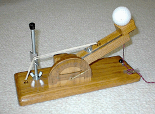
This experiment was conducted by a team of students on a catapult, a table-top wooden device used to teach design of experiments and statistical process control. The catapult has several controllable factors and a response easily measured in a classroom setting. It has been used for over 10 years in hundreds of classes.
Description of Experiment: Response and Factors
The experiment has five factors that might affect the distance the golf ball travels
Purpose: To determine the significant factors that affect the distance the ball is thrown by the catapult, and to determine the settings required to reach three different distances (30, 60 and 90 inches).
Response Variable: The distance in inches from the front of the catapult to the spot where the ball lands. The ball is a plastic golf ball.
Number of observations: 20 (a \(2^{5-1}\) resolution V design with 4 center points).
Variables:
- Response Variable Y = distance
- Factor 1 = band height (height of the pivot point for the rubber bands, levels were 2.25 and 4.75 inches with a centerpoint level of 3.5)
- Factor 2 = start angle (location of the arm when the operator releases, starts the forward motion of the arm, levels were 0 and 20 degrees with a centerpoint level of 10 degrees)
- Factor 3 = rubber bands (number of rubber bands used on the catapult, levels were 1 and 2 bands)
- Factor 4 = arm length (distance the arm is extended, levels were 0 and 4 inches with a centerpoint level of 2 inches)
- Factor 5 = stop angle (location of the arm where the forward motion of the arm is stopped and the ball starts flying, levels were 45 and 80 degrees with a centerpoint level of 62 degrees)
Design matrix and responses (in run order)
The design matrix appears below in (randomized) run order.
distance height start bands length stop order
   28.00   3.25     0    1      0   80     1
   99.00      4    10    2      2   62     2
  126.50   4.75    20    2      4   80     3
  126.50   4.75     0    2      4   45     4
   45.00   3.25    20    2      4   45     5
   35.00   4.75     0    1      0   45     6
   45.00      4    10    1      2   62     7
   28.25   4.75    20    1      0   80     8
   85.00   4.75     0    1      4   80     9
    8.00   3.25    20    1      0   45    10
   36.50   4.75    20    1      4   45    11
   33.00   3.25     0    1      4   45    12
   84.50      4    10    2      2   62    13
   28.50   4.75    20    2      0   45    14
   33.50   3.25     0    2      0   45    15
   36.00   3.25    20    2      0   80    16
   84.00   4.75     0    2      0   80    17
   45.00   3.25    20    1      4   80    18
   37.50      4    10    1      2   62    19
  106.00   3.25     0    2      4   80    20
One discrete factor
Note that four of the factors are continuous, and one, number of rubber bands, is discrete. Due to the presence of this discrete factor, we actually have two different centerpoints, each with two runs. Runs 7 and 19 are with one rubber band, and the center of the other factors, while runs 2 and 13 are with two rubber bands and the center of the other factors.
Five confirmatory runs
After analyzing the 20 runs and determining factor settings needed to achieve predicted distances of 30, 60 and 90 inches, the team was asked to conduct five confirmatory runs at each of the derived settings.
Analysis of the Experiment
Step 1: Look at the data
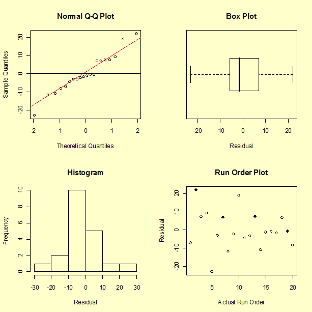
Histogram, box plot, normal probability plot, and run order plot of the response
We start by plotting the data several ways to see if any trends or anomalies appear that would not be accounted for by the models.
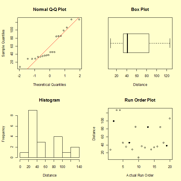
We can see the large spread of the data and a pattern to the data that should be explained by the analysis. The run order plot does not indicate an obvious time sequence. The four highlighted points in the run order plot are the center points in the design. Recall that runs 2 and 13 had two rubber bands and runs 7 and 19 had one rubber band. There may be a slight aging of the rubber bands in that the second center point resulted in a distance that was a little shorter than the first for each pair.
Plots of responses versus factor columns
Next look at the plots of responses sorted by factor columns.
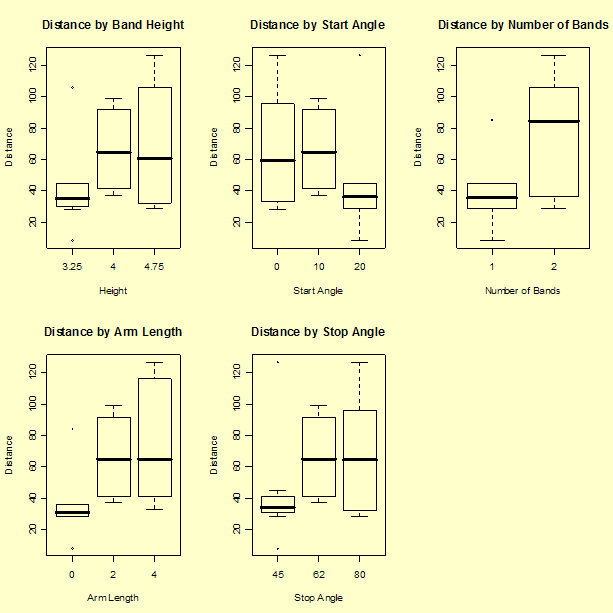
Several factors appear to change the average response level and most have large spread at each of the levels.
Step 2: Create the theoretical model
The resolution V design can estimate main effects and all two-factor interactions
With a resolution V design we are able to estimate all the main effects and all two-factor interactions without worrying about confounding. Therefore, the initial model will have 16 terms: the intercept term, the 5 main effects, and the 10 two-factor interactions.
Step 3: Create the actual model from the data
Variable coding
Note we have used the orthogonally coded columns for the analysis, and have abbreviated the factor names as follows:
- Height (h) = band height
- Start (s) = start angle
- Bands (b) = number of rubber bands
- Stop (e) = stop angle
- Length (l) = arm length
Trial model with all main factors and two-factor interactions
The results of fitting the trial model that includes all main factors and two-factor interactions follow.
Source      Estimate  Std. Error  t value  Pr(>|t|)
---------   --------  ----------  -------  --------
Intercept    57.5375      2.9691   19.378  4.18e-05 ***
h            13.4844      3.3196    4.062   0.01532 *
s           -11.0781      3.3196   -3.337   0.02891 *
b            19.4125      2.9691    6.538   0.00283 **
l            20.1406      3.3196    6.067   0.00373 **
e            12.0469      3.3196    3.629   0.02218 *
h*s          -2.7656      3.3196   -0.833   0.45163
h*b           4.6406      3.3196    1.398   0.23467
h*l           4.7031      3.3196    1.417   0.22950
h*e           0.1094      3.3196    0.033   0.97529
s*b          -3.1719      3.3196   -0.955   0.39343
s*l          -1.1094      3.3196   -0.334   0.75502
s*e           2.6719      3.3196    0.805   0.46601
b*l           7.6094      3.3196    2.292   0.08365 .
b*e           2.8281      3.3196    0.852   0.44225
l*e           3.1406      3.3196    0.946   0.39768

Significance codes:  0 '***' 0.001 '**' 0.01 '*' 0.05 '.' 0.1 ' ' 1

Residual standard error:  13.28, based on 4 degrees of freedom
Multiple R-squared:  0.9709
Adjusted R-squared:  0.8619
F-statistic:  8.905, based on 15 and 4 degrees of freedom
p-value: 0.02375
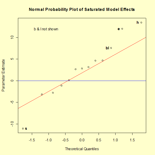
Use p-values and a normal probability plot to help select significant effects
The model has a good \(R^2\) value, but the fact that \(R^2\) adjusted is considerably smaller indicates that we undoubtedly have some terms in our model that are not significant. Scanning the column of p-values (labeled Pr(>|t|)) for small values shows five significant effects at the 0.05 level and another one at the 0.10 level.
A normal probability plot of effects is a useful graphical tool to determine significant effects. The graph below shows that there are nine terms in the model that can be assumed to be noise. That would leave six terms to be included in the model. Whereas the output above shows a p-value of 0.0836 for the interaction of Bands (b) and Length (l), the normal plot suggests we treat this interaction as significant.
Refit using just the effects that appear to matter
Remove the non-significant terms from the model and refit to produce the following analysis of variance table.
Source           Df Sum of Sq  Mean Sq   F value   Pr(>F)
-----------      -- ---------  -------   -------   ------
Model             6  22148.55   3691.6
Total error      13   2106.99    162.1     22.77  3.5e-06

Lack-of-fit      11   1973.74    179.4
Pure error        2    133.25     66.6      2.69   0.3018

Residual standard error:  12.73 based on 13 degrees of freedom
Multiple R-squared:  0.9131
Adjusted R-squared:  0.873
\(R^2\) is OK and there is no significant model "lack of fit"
The \(R^2\) and \(R^2\) adjusted values are acceptable. The ANOVA table shows us that the model is significant, and the lack-of-fit test is not significant. Parameter estimates are below.
Source      Estimate  Std. Error  t value  Pr(>|t|)
---------   --------  ----------  -------  --------
Intercept     57.537       2.847   20.212  3.33e-11 ***
h             13.484       3.183    4.237   0.00097 ***
s            -11.078       3.183   -3.481   0.00406 **
b             19.412       2.847    6.819  1.23e-05 ***
l             20.141       3.183    6.328  2.62e-05 ***
e             12.047       3.183    3.785   0.00227 **
b*l            7.609       3.183    2.391   0.03264 *

Significance codes:  0 '***' 0.001 '**' 0.01 '*' 0.05 '.' 0.1 ' ' 1
Step 4: Test the model assumptions using residual graphs (adjust and simplify as needed)
Diagnostic residual plots
To examine the assumption that the residuals are approximately normally distributed, are independent, and have equal variances, we generate four plots of the residuals: a normal probability plot, box plot, histogram, and a run-order plot of the residuals. In the run-order plot, the highlighted points are the centerpoint values. Recall that run numbers 2 and 13 had two rubber bands while run numbers 7 and 19 had only one rubber band.
The residuals do appear to have, at least approximately, a normal distribution.
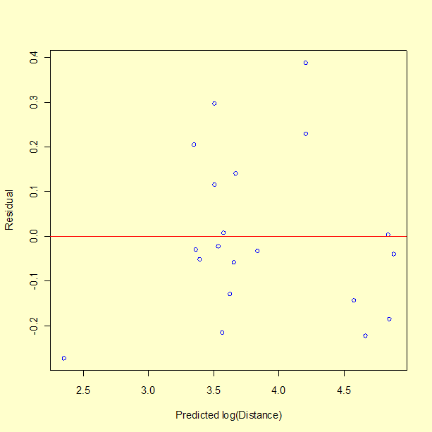
Plot of residuals versus predicted values
Next we plot the residuals versus the predicted values.
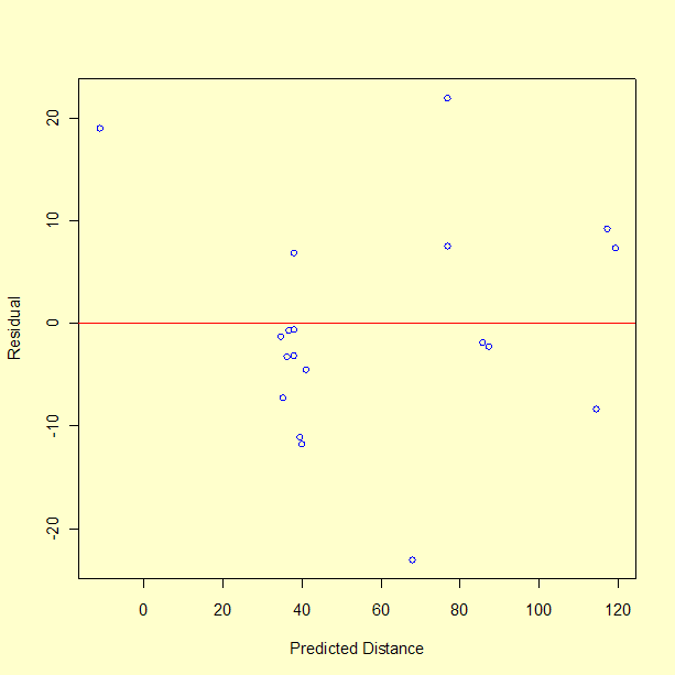
There does not appear to be a pattern to the residuals. One observation about the graph, from a single point, is that the model performs poorly in predicting a short distance. In fact, run number 10 had a measured distance of 8 inches, but the model predicts -11 inches, giving a residual of 19 inches. The fact that the model predicts an impossible negative distance is an obvious shortcoming of the model. We may not be successful at predicting the catapult settings required to hit a distance less than 25 inches. This is not surprising since there is only one data value less than 28 inches. Recall that the objective is to achieve distances of 30, 60, and 90 inches.
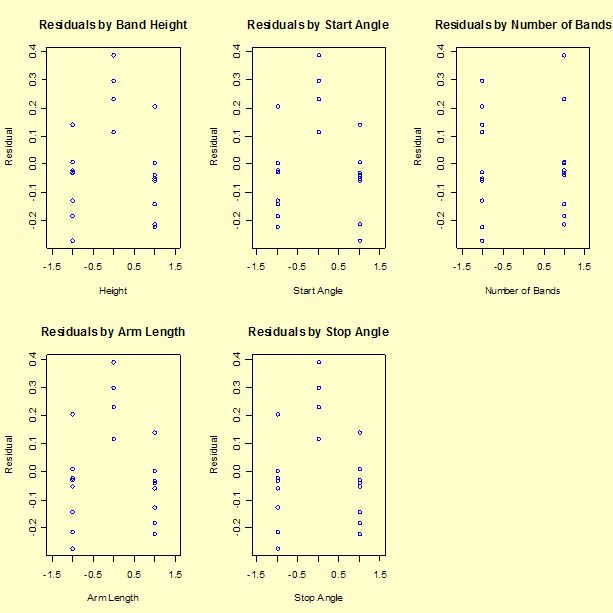
Plots of residuals versus the factor variables
Next we look at the residual values versus each of the factors.
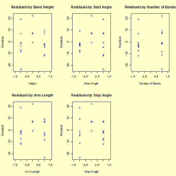
The residual graphs are not ideal, although the model passes the lack-of-fit test
Most of the residual graphs versus the factors appear to have a slight "frown" on the graph (higher residuals in the center). This may indicate a lack of fit, or sign of curvature at the centerpoint values. The lack-of-fit test, however, indicates that the lack of fit is not significant.
Consider a transformation of the response variable to see if we can obtain a better model
At this point, since there are several unsatisfactory features of the model we have fit and the resultant residuals, we should consider whether a simple transformation of the response variable (Y = "Distance") might improve the situation.
There are at least two good reasons to suspect that using the logarithm of distance as the response might lead to a better model.
- A linear model fit to \(\ln(Y)\) will always predict a positive distance when converted back to the original scale for any possible combination of X factor values.
- Physical considerations suggest that a realistic model for distance might require quadratic terms since gravity plays a key role — taking logarithms often reduces the impact of non-linear terms.
To see whether using \(\ln(Y)\) as the response leads to a more satisfactory model, we return to step 3.
Step 3a: Fit the full model using ln(Y) as the response
First a main effects and two-factor interaction model is fit to the log distance responses
Proceeding as before, using the coded values of the factor levels and the natural logarithm of distance as the response, we obtain the following parameter estimates.
Source      Estimate  Std. Error  t value  Pr(>|t|)
---------   --------  ----------  -------  --------
(Intercept)  3.85702     0.06865   56.186  6.01e-07 ***
h            0.25735     0.07675    3.353   0.02849 *
s           -0.24174     0.07675   -3.150   0.03452 *
b            0.34880     0.06865    5.081   0.00708 **
l            0.39437     0.07675    5.138   0.00680 **
e            0.26273     0.07675    3.423   0.02670 *
h*s         -0.02582     0.07675   -0.336   0.75348
h*b         -0.02035     0.07675   -0.265   0.80403
h*l         -0.01396     0.07675   -0.182   0.86457
h*e         -0.04873     0.07675   -0.635   0.55999
s*b          0.00853     0.07675    0.111   0.91686
s*l          0.06775     0.07675    0.883   0.42724
s*e          0.07955     0.07675    1.036   0.35855
b*l          0.01499     0.07675    0.195   0.85472
b*e         -0.01152     0.07675   -0.150   0.88794
l*e         -0.01120     0.07675   -0.146   0.89108

Signif. codes:  0 '***' 0.001 '**' 0.01 '*' 0.05 '.' 0.1 ' ' 1

Residual standard error:  0.307 based on 4 degrees of freedom
Multiple R-squared:  0.9564
Adjusted R-squared:  0.7927
F-statistic:  5.845 based on 15 and 4 degrees of freedom
p-value:  0.0502
A simpler model with just main effects has a satisfactory fit
Examining the p-values of the 16 model coefficients, only the intercept and the 5 main effect terms appear significant. Refitting the model with just these terms yields the following results.
Source           Df Sum of Sq  Mean Sq   F value    Pr(>F)
-----------      -- ---------  -------   -------    ------
Model             5   8.02079   1.60416   36.285   1.6e-07
Total error      14   0.61896   0.04421

Lack-of-fit      12   0.58980   0.04915
Pure error        2   0.02916   0.01458    3.371    0.2514


Source      Estimate  Std. Error  t value  Pr(>|t|)
---------   --------  ----------  -------  --------
Intercept    3.85702     0.04702   82.035   < 2e-16 ***
h            0.25735     0.05257    4.896  0.000236 ***
s           -0.24174     0.05257   -4.599  0.000413 ***
b            0.34880     0.04702    7.419  3.26e-06 ***
l            0.39437     0.05257    7.502  2.87e-06 ***
e            0.26273     0.05257    4.998  0.000195 ***

Signif. codes:  0 '***' 0.001 '**' 0.01 '*' 0.05 '.' 0.1 ' ' 1

Residual standard error:  0.2103 based on 14 degrees of freedom
Multiple R-squared:  0.9284
Adjusted R-squared:  0.9028
This is a simpler model than previously obtained in Step 3 (no interaction term). All the terms are highly significant and there is no indication of a significant lack of fit.
We next look at the residuals for this new model fit.
Step 4a: Test the (new) model assumptions using residual graphs (adjust and simplify as needed)
Normal probability plot, box plot, histogram, and run-order plot of the residuals
The following normal plot, box plot, histogram and run-order plot of the residuals shows no problems.
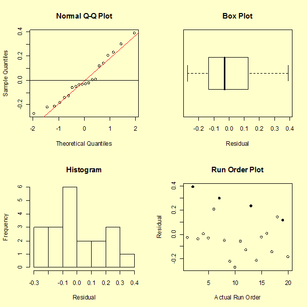
Residuals plotted versus run order again show a possible slight decreasing trend (rubber band fatigue?).
Plot of residuals versus predicted ln(Y) values
A plot of the residuals versus the predicted \(\ln(Y)\) values looks reasonable, although there might be a tendency for the model to overestimate slightly for high predicted values.
Plot of residuals versus the factor variables
Next we look at the residual values versus each of the factors.
The residuals for the main effects model (fit to natural log of distance) are reasonably well behaved
These plots still appear to have a slight "frown" on the graph (higher residuals in the center). However, the model is generally an improvement over the previous model and will be accepted as possibly the best that can be done without conducting a new experiment designed to fit a quadratic model.
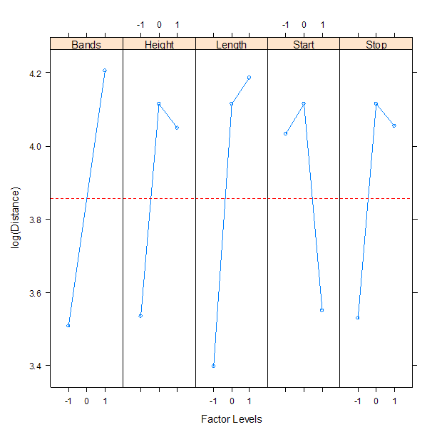
Step 5: Use the results to answer the questions in your experimental objectives
Final step: Predict the settings that should be used to obtain desired distances
Based on the analyses and plots, we can select factor settings that maximize the log-transformed distance. Translating from "-1", "0", and "+1" back to the actual factor settings, we have: band height at "0" or 3.5 inches; start angle at "0" or 10 degrees; number of rubber bands at "1" or 2 bands; arm length at "1" or 4 inches, and stop angle at "0" or 80 degrees.
"Confirmation" runs were successful
In the confirmatory runs that followed the experiment, the team was successful at hitting all three targets, but did not hit them all five times. The model discovery and fitting process, as illustrated in this analysis, is often an iterative process.